4.10. KNN Classification#
K-nearest neighbours (KNN) classification is a commonly used machine learning algorithm for classification (predicting classes/categories), and follows the same principles as KNN regression, but instead of making a prediction using the average value of the neighbours, it predicts by taking the majority class of the neighbours.
4.10.1. KNN Classification In 1D#
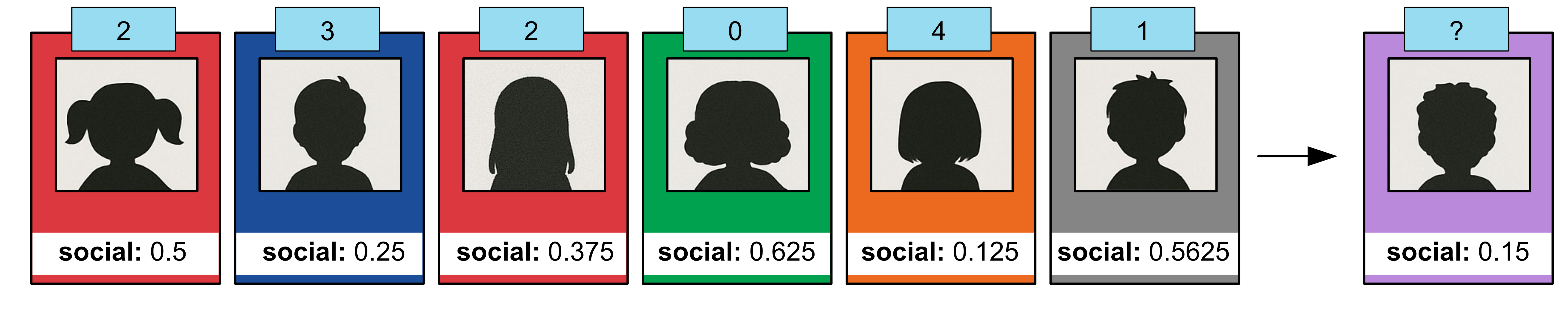
Consider the following dataset containing voter views. There are 5 parties the voters can vote for:
0: The green party
1: The grey party
2: The red party
3: The blue party
4: The orange party
The social score is a number between 0 and 1, which indicates the voter’s social views. Lower values indicate conservative views and higher numbers indicate progressive views.
Social |
Vote |
|---|---|
0.5 |
2 |
0.25 |
3 |
0.375 |
2 |
0.625 |
0 |
0.625 |
1 |
0.5 |
2 |
0.375 |
3 |
0.125 |
4 |
0.875 |
0 |
0.3125 |
3 |
0.5625 |
2 |
0.5625 |
1 |
0.75 |
0 |
0.5 |
2 |
0.25 |
3 |
If we were to plot out the data it would look like this.
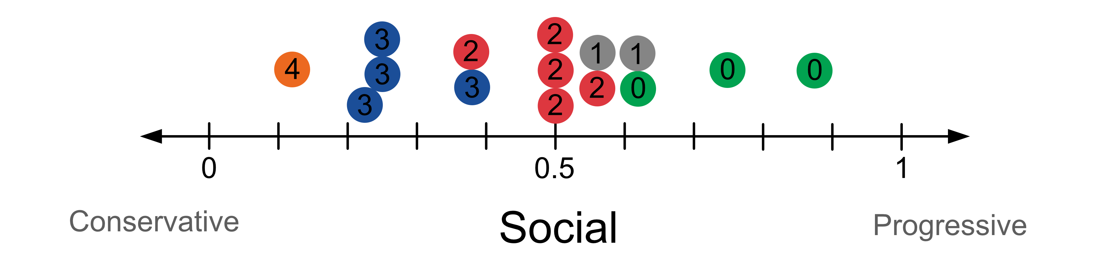
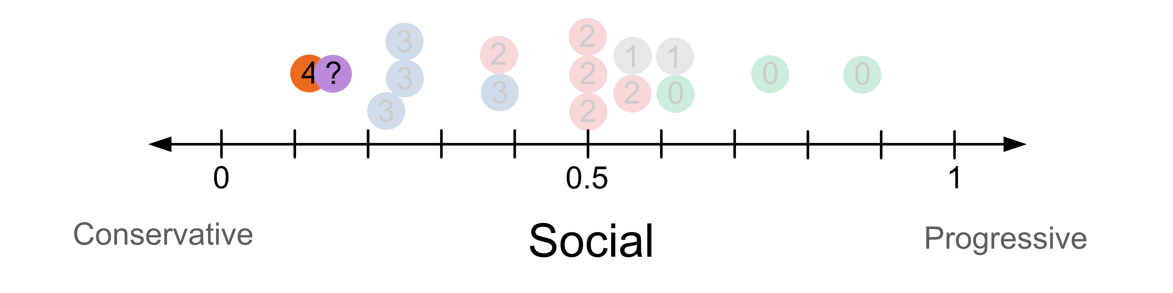
Now let’s try to classify our test sample who has a social score of 0.15. For k = 1, we look at the vote of the closest neighbour and use this to predict how the person will vote. In this case we predict they vote for group 4, the orange party.
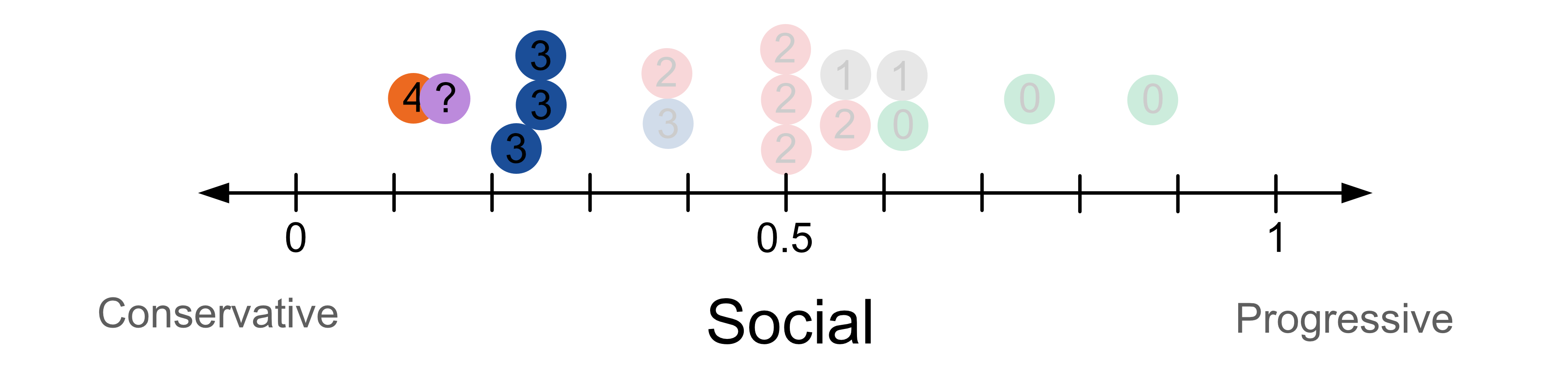
If we were to change k to k=4, we have 4 neighbours, one voting for group 4, the orange party and three voting for group 3, the blue party. In this case we predict with the majority class. In this case we predict they vote for group 3, the blue party.
4.10.2. KNN Classification In 2D#
We have now expanded our voter views dataset so that in addition to each voter’s social score we also have their economic score. We have 50 samples in total, but in the table below we just show the first 15.
Economic |
Social |
Vote |
|---|---|---|
0.5 |
0.5 |
2 |
0.625 |
0.25 |
3 |
0.375 |
0.375 |
2 |
0.375 |
0.625 |
0 |
0.625 |
0.625 |
1 |
0.625 |
0.5 |
2 |
0.75 |
0.375 |
3 |
0.75 |
0.125 |
4 |
0.5 |
0.875 |
0 |
0.5625 |
0.3125 |
3 |
0.75 |
0.5625 |
2 |
0.5 |
0.5625 |
1 |
0.1875 |
0.75 |
0 |
0.4375 |
0.5 |
2 |
0.8125 |
0.25 |
3 |
If we plot out the data it would look like this.
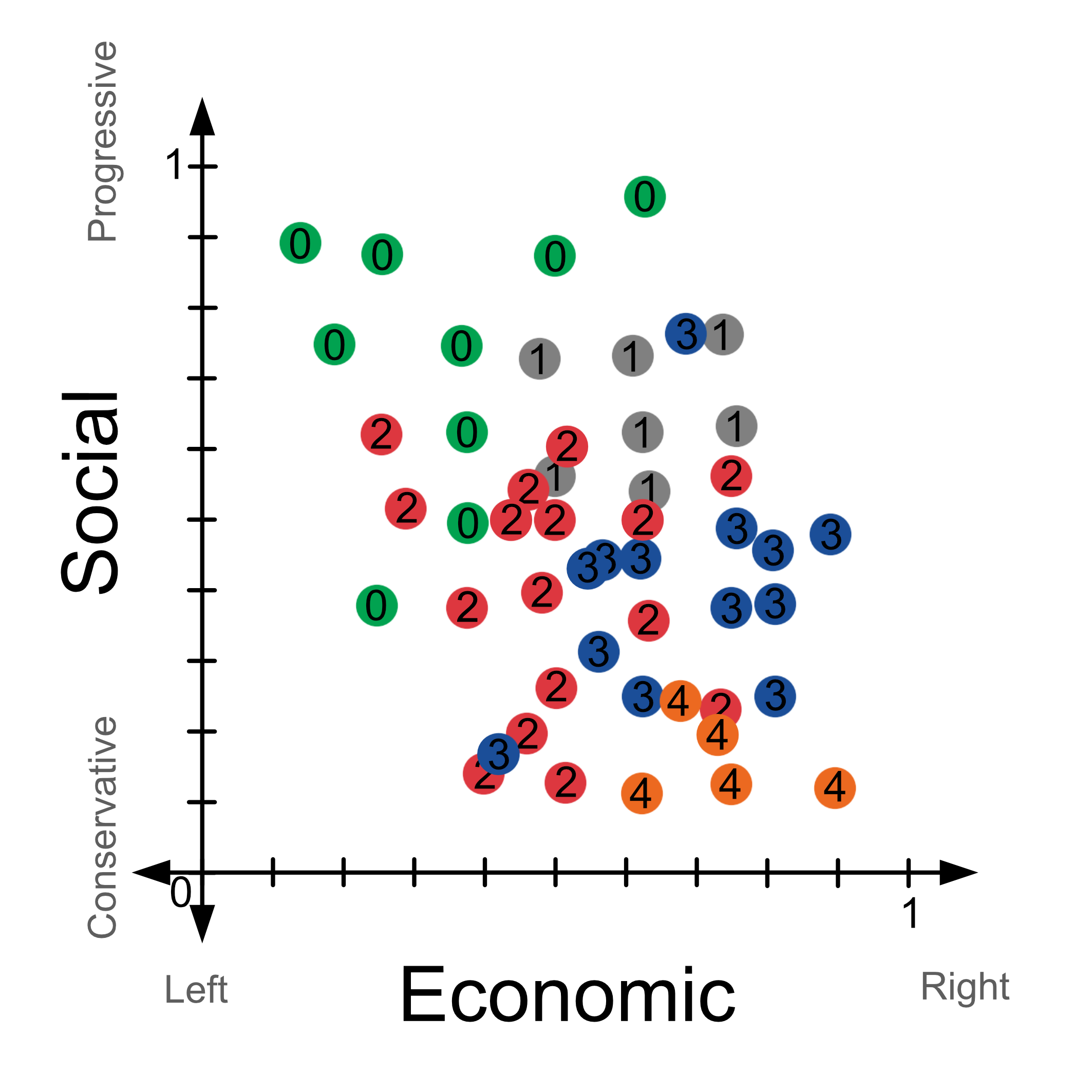
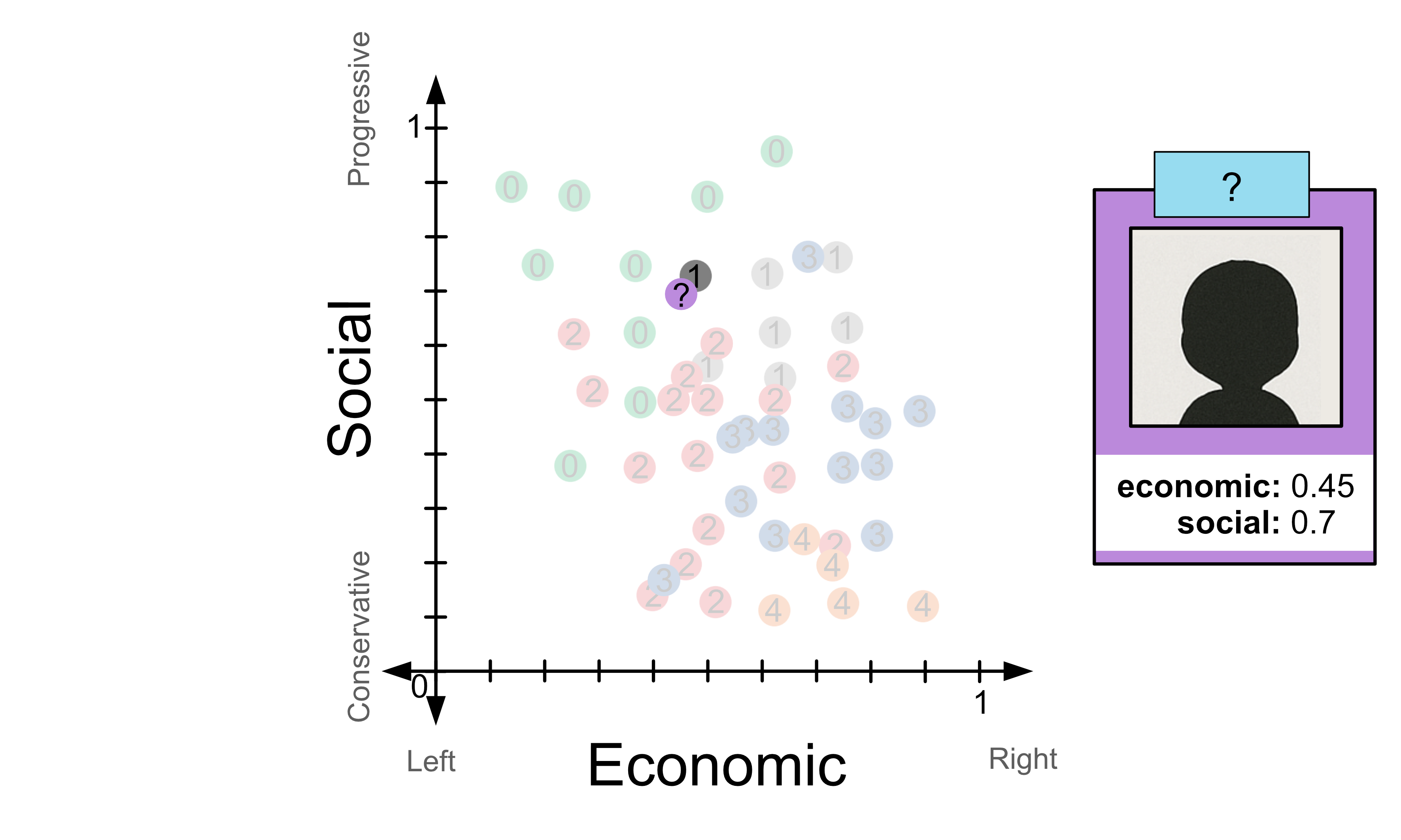
Let’s try to predict how a someone with an economic score of 0.45 and a social score of 0.7 would vote. If we look at the example where k=1, i.e. the closest neighbour we would predict that the person would vote for party 1, the grey party.
What if we used k=4 instead? Then we’d need to look at the 4 closest neighbours and look for the majority class. In this case, that is part 0, the green party. So for k=4, we would predict that the person would vote for party 0, the green party.
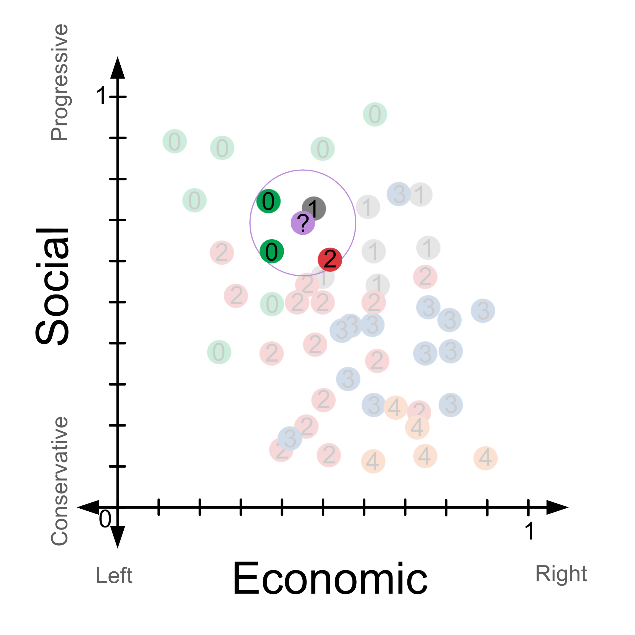
In the event that there is a tie for the majority class we pick randomly between the two classes.