2.5. Extension: Selecting The Polynomial Degree

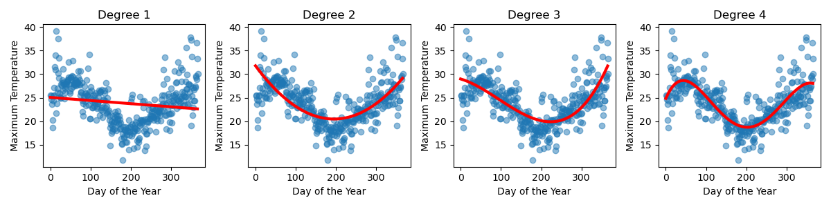
Sometimes it’s clear what polynomial degree you should select for your data. For example, our Sydney temperature data needed to be at least degree 4 to have enough ‘wiggles’ to capture the shape of the data.

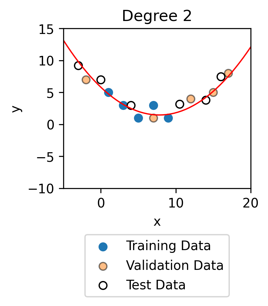
But consider the following data.

Based on this data, and this data alone, it’s not necessarily clear which of these models is actually capturing the true trends of this small dataset.

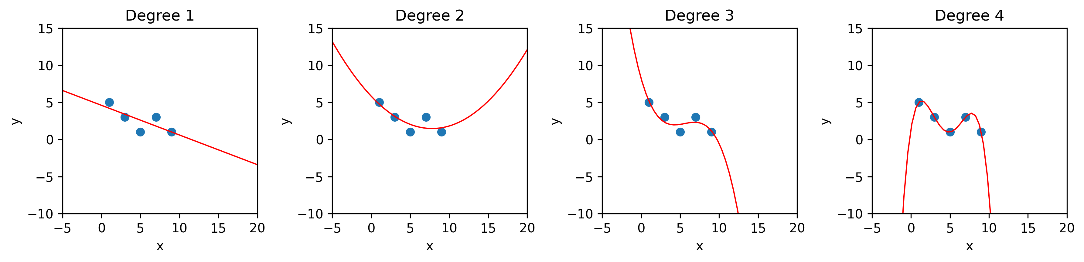
Comparing the mean squared errors (MSEs) we would find the polynomial of degree 4 performs best.

Degree	MSE
1	0.96
2	0.73
3	0.41
4	0

However, it’s not actually fair to compare the performance of different types of models on the data the models have already seen. This is because a polynomial of higher degree has more ‘wiggles’ and create more curves, so it will always be able to fit the data better than a lower degree model. You will notice that in the table above the MSE decreases as the model degree increases.

Often what we care about is how the model performs on new data.

We typically break our data up into:

• training data: Used to fit the model (it’s what you provide when you call .fit()). This is what the model ‘sees’ as it’s trying to figure out the the shape of the curve it should produce.

• validation data: Used to determine the degree of the polynomial that should be used to fit the data.

• test data: Used to estimate the performance of the final model.

It’s really important that all three data sets are completely different, e.g. none of the test data contains any of the training data and not of the validation data contains any of the test data. This is because we care about how our models perform on new data, data it hasn’t already seen. It’s like when designing a final exam for students. It’s important that the exam contains new questions that the students haven’t already seen.

Now let’s see how our models perform on the validation data.

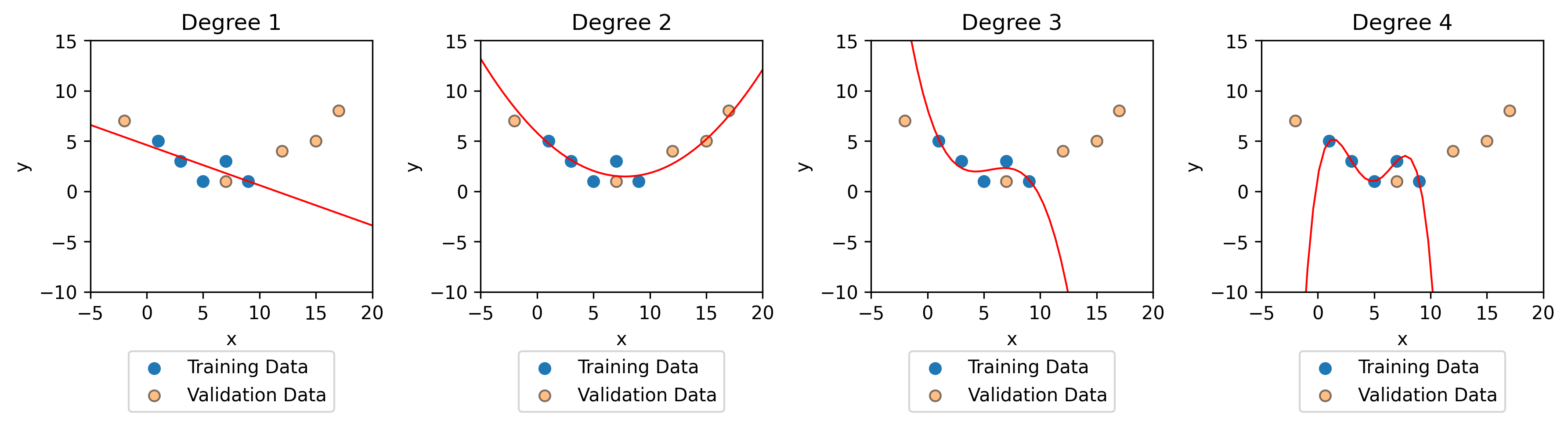
Comparing the validation MSEs we can see that the polynomial of degree 2 performs the best on the validation data. This means that we expect the polynomial of degree 2 to perform best on new data.

Degree	Training MSE	Validation MSE
1	0.96	33.2
2	0.73	0.78
3	0.41	1174
4	0	98944

You can think of validation data as ‘practice test data’. But at the end of the day, we still want to know how well our data will do on completely new data. Remember that we’ve already seen the validation data when we selected the model degree, so now we introduce some test data. At this point, you don’t have to worry about the other polynomial regression we’ve built.

Degree	Training MSE	Validation MSE	Test MSE
2	0.73	0.78	0.86

In general, the model will tend to perform best on the training data because this is data it has seen and is given the y value for, just like how a student would perform best on questions they might have seen the answers to. The model will tend to perform similarly well on the validation and test data. If there is not much data, the difference in performance on the various training sets comes down to a bit of ‘luck’.

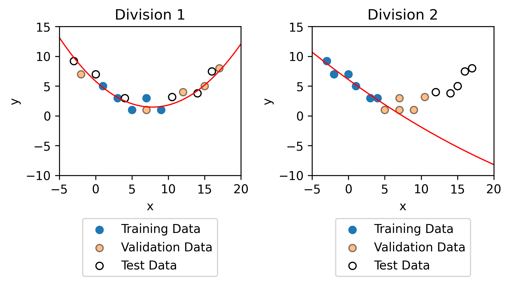
It is important, however that the training data, the validation data and the test data all try to capture the general trends of the data. For example, with the exact same data, but a different division between the training, validation and test data (as shown below).

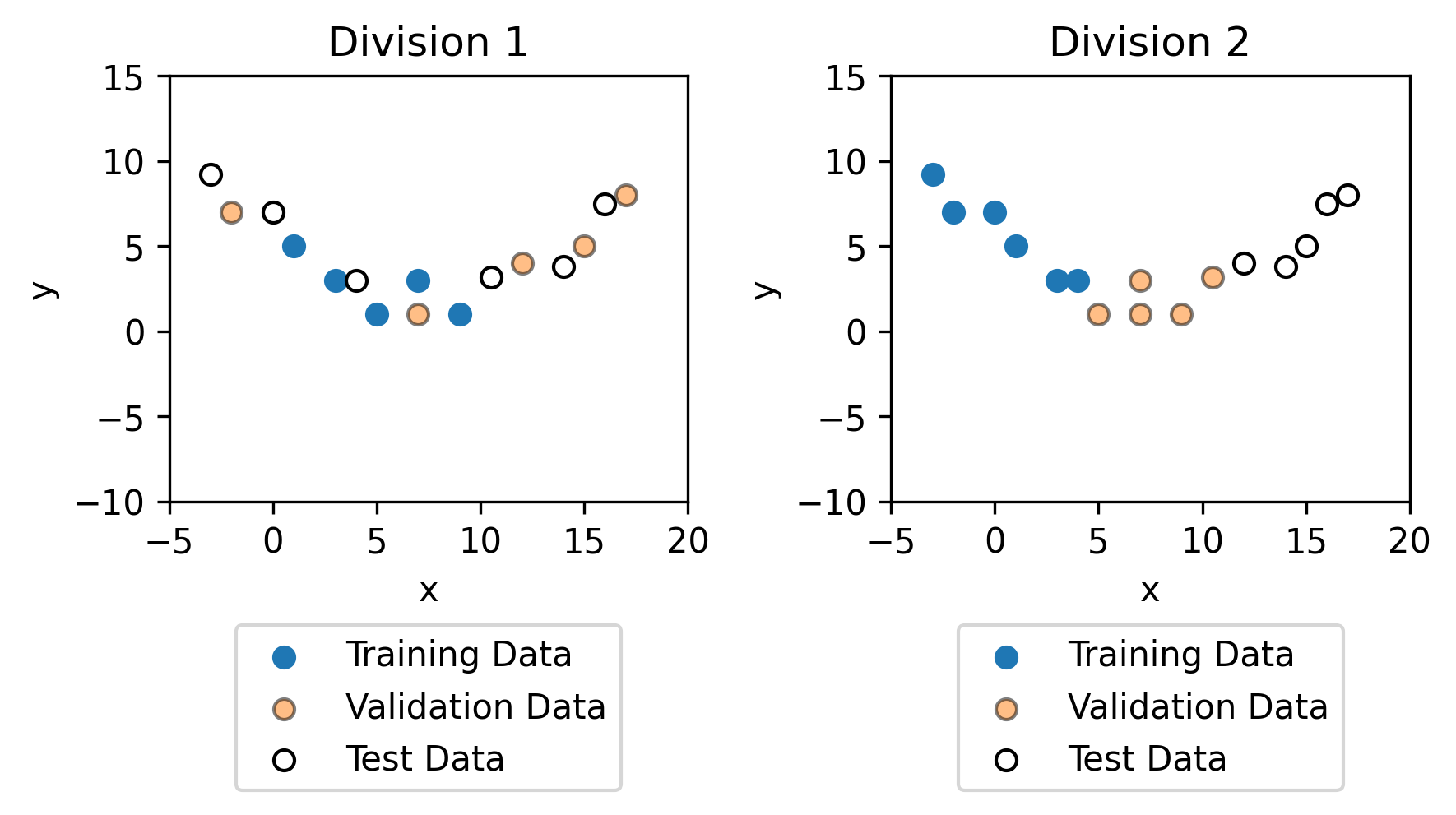
Fitting models to the training data results in completely different models. As you can see, the training data in division 2 is not representative on the whole dataset, which is why the model for division 2 is not representative on the dataset.