Extension: Further Classification Metrics

2.10. Extension: Further Classification Metrics#

2.10.1. Confusion Matrices#

When it comes to classification models, a useful way to evaluate the performance of the model is to calculate the following:

True positives (TP): number of samples predicted to be in class 1 that are actually in class 1
True negatives (TN): number of samples predicted to be in class 0 that are actually in class 0
False positives (FP): number of samples that are predicted to be in class 1 the are not in class 1
False negatives (FN): number of samples that are predicted to be in class 0 that are not in class 0

These values are represented visually by using them to construct a table called a confusion matrix. This matrix arranges the TP, TN, FP and FN values in the following way:

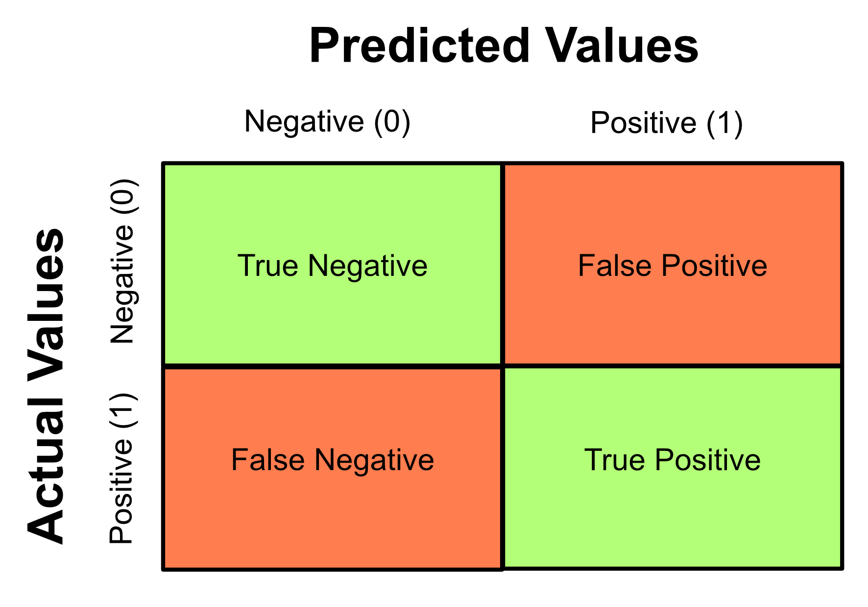
Note

There isn’t a convention for which axes should present the actual or predicted values, so note that you may see other confusion matrices with the axes switched.

A model that performs well will have high true negative and true positive values and low false positive and false negative values - this is because it will have correctly identified most of negative and positive classes with little error. Therefore, the ideal confusion matrix will have large values along the diagonal. This means that all the data has been correctly classified.

It is important to understand the implications of the FP and FN values. For example:

You have Covid-19 but a Covid test comes up as negative → false negative
You are not pregnant but a pregnancy test comes up as positive → false positive

As you can see, FP and FN results can have serious consequences! As classification algorithms are increasingly used in new applications, assessing the impacts of FP and FN cases is always important.

You can generate a confusion matrix using the sklearn library.

from sklearn.metrics import confusion_matrix

This allows you to use the confusion_matrix function:

confusion_matrix(actual_classes, predicted_classes)

from sklearn.metrics import confusion_matrix

predicted = [1, 0, 0, 0, 1, 1, 1, 0, 1, 0, 0, 0, 1, 1]
actual = [1, 1, 0, 0, 1, 1, 1, 0, 0, 0, 0, 1, 0, 0]
print(confusion_matrix(actual, predicted))

2.10.2. Precision, Recall and F1 Score#

Sometimes we worry more about false negatives and sometimes we worry more about false positives.

For example, with a Covid-19 test, we’re worried more about false negatives than false positives.

Consequences of a false positive: a person believes they have covid when they don’t and that individual stays home an isolates.
Consequences of a false negative: a person believe they do not have covid when they do and that individual spreads covid to other people.

Other commonly used metrics include precision, recall and F1 score.

Precision: of the samples we predicted to be positive, how many were actually positive? i.e. proportion of relevant data our model predicted as being relevant

\[\text{Precision} = \cfrac{TP}{\text{Classified positive}} = \cfrac{TP}{TP + FP}\]

Recall: of the samples that are actually positive, how many were classified as positive? i.e. how well our model was able to find the relevant data

\[\text{Recall} = \cfrac{TP}{\text{Actually positive}} = \cfrac{TP}{TP + FN}\]

In certain situations, we want to maximise either precision or recall. In our Covid-19 example we want to minimise false negatives. You will notice that false negatives appear in the denominator of the recall metric. To minimise false negatives we want to maximise recall.

F1 score: the harmonic mean of precision and recall.

\[\text{F}_1 = \cfrac{2}{\text{recall}^{-1}+\text{precision}^{-1}} = \cfrac{2\times\text{precision}\times\text{recall}}{\text{precision} + \text{recall}}\]

The F1 score can be used as a metric if your context has no preference to either recall or precision.

The confusion_matrix function we learned earlier can return us the TN, FP, FN and TP values if we use flatten() to convert the 2D array into a 1D array as follows:

tn, fp, fn, tp = confusion_matrix(actual_classes, predicted_classes).flatten()

from sklearn.metrics import confusion_matrix

predicted = [1, 0, 0, 0, 1, 1, 1, 0, 1, 0, 0, 0, 1, 1]
actual = [1, 1, 0, 0, 1, 1, 1, 0, 0, 0, 0, 1, 0, 0]
tn, fp, fn, tp = confusion_matrix(actual, predicted).flatten()

precision = tp / (tp + fp)
recall = tp / (tp + fn)
f1 = (2 * precision * recall) / (precision + recall)

print("Precision: {:.2f}".format(precision))
print("Recall: {:.2f}".format(recall))
print("F1: {:.2f}".format(f1))

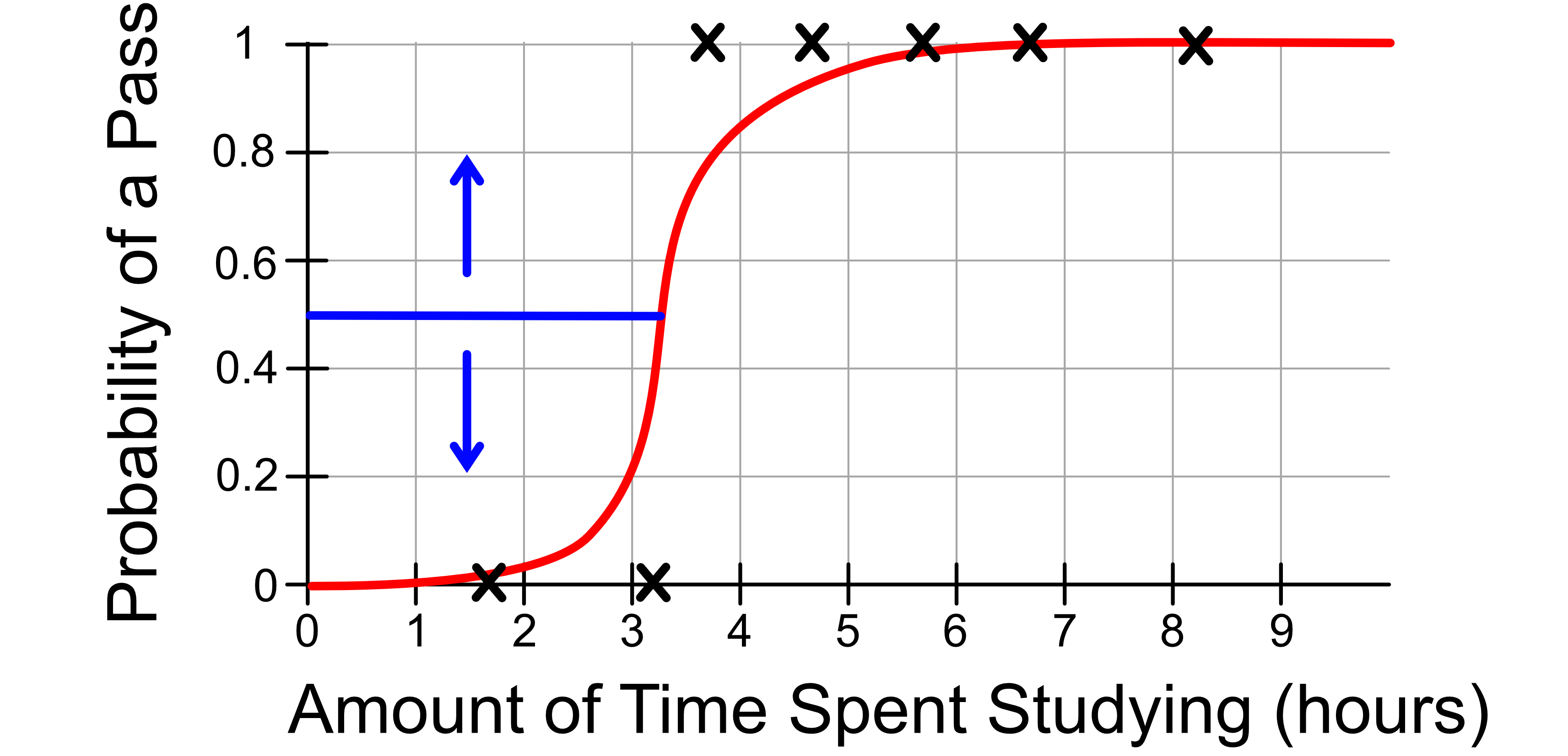
2.10.3. Probability Threshold#

By default:

If the probability of class 1 is greater than 0.5, we predict class 1
If the probability of class 1 is less than 0.5, we predict class 0

We can change the performance of our model by changing the threshold at which we make the decision.

Returning again with our Covid-19 example, we might adjust our threshold to ‘err on the side of caution’. We might change our decision making process so that:

If the probability of class 1 is greater than 0.4, we predict class 1, i.e. that the patient has Covid
If the probability of class 1 is less than 0.4, we predict class 0, i.e. that the patient does not have Covid

This will increase our false positives and decrease our false negatives.

Code Challenge: Extension: Calculate Metrics

We previously used our logistic regression model to predict whether it will rain based on the number of sunshine hours seen in the previous day using the following test data.

Sunshine	RainTomorrow
2.2	0
5.0	0
7.3	0
3.2	1
1.7	1
4.1	0
5.5	1

Instructions

Copy and paste in your code from Predicting With A Logistic Regression Model using rain.csv.
Create an array storing the actual classes of each test sample
Calculate the precision, recall and F1 score of the predictions the model made on the test data

Your output should look like this:

Precision: X.XX
Recall: X.XX
F1: X.XX