2.9. Predicting With A Logistic Regression Model

2.9.1. Class Prediction

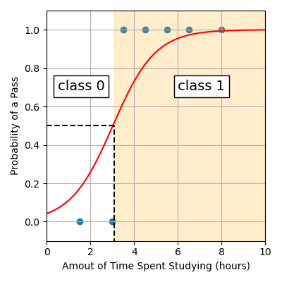
We can make predictions using our linear regression model by estimating the \(y\) value for a given \(x\) value.

For example, returning to our study example, we can see students studying more than ~3.1 hours are expected to pass (class 1) since the curve of the logistic function sits at a probability greater than 0.5. Whereas students studying less than ~3.1 hours are expected to fail (class 0).

Alternatively, our sklearn LogisticRegression model comes with an in-built function that allows us to make a prediction.

Note

x must be a 2D array with n rows, one for each sample we want to predict on and 1 column. An easy way to achieve this is to use .reshape(-1, 1).

Here’s a full example using the test data 2.5, 3.2 and 7.

from sklearn.linear_model import LogisticRegression
import pandas as pd
import numpy as np

# Load data
data = pd.read_csv("pass_fail.csv")
x = data["Time Spent Studying (hours)"].to_numpy()
y = data["Exam Result"].to_numpy()

# Build logistic regression model
logistic_reg = LogisticRegression()
logistic_reg.fit(x.reshape(-1, 1), y)

x_test = np.array([2.5, 3.2, 7])
print(logistic_reg.predict(x_test.reshape(-1, 1)))

Output

[0 1 1]

Here are the predictions the model makes:

Time Spent Studying (hours)	Exam (Fail 0/Pass 1)
2.5	0
3.2	1
7	1

The first student who studied 2.5 hours is predicted to fail and the students who studied 3.2 and 7 hours are predicted to pass.

2.9.2. Class Probability

In addition to the class, we can show the probability of being in each class.

log_reg.predict_proba(x)

The first column gives the probability of the sample being in class 0 and the second column gives us the probability of being in class 1. The probability curve of class 1 is actually what we see when we visualise our model. We can extract out the second column using [:, 1]. The : means ‘select all rows’ and the 1 means ‘select column 1’.

log_reg.predict_proba(x)[:, 1]

This means instead of calculating \(y\) values using the model equation \(y = \cfrac{1}{1+e^{-(\beta_0 + \beta_1x)}}\) (as shown below):

x_model = np.linspace(0, 10, 50)
y_model = 1 / (1 + np.exp(-(beta0 + beta1 * x_model)))

We can use .predict_proba(). Note that we still need to reshape the data.

x_model = np.linspace(0, 10, 50)
y_model = logistic_reg.predict_proba(x_model.reshape(-1, 1))[:, 1]

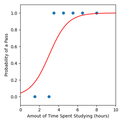
We have updated the code below to provide a full example.

from sklearn.linear_model import LogisticRegression
import matplotlib.pyplot as plt
import pandas as pd
import numpy as np

# Load data
data = pd.read_csv("pass_fail.csv")
x = data["Time Spent Studying (hours)"].to_numpy()
y = data["Exam Result"].to_numpy()

# Build logistic regression model
logistic_reg = LogisticRegression()
logistic_reg.fit(x.reshape(-1, 1), y)

# Create x and y values to visualise the model function
x_model = np.linspace(0, 10, 50)
y_model = logistic_reg.predict_proba(x_model.reshape(-1, 1))[:, 1]

plt.figure(figsize=(4, 4))
plt.scatter(x, y)  # Data
plt.plot(x_model, y_model, color="red")  # Model
plt.xlabel("Amout of Time Spent Studying (hours)")
plt.ylabel("Probability of a Pass")
plt.xlim([0, 10])
plt.ylim([-0.1, 1.1])
plt.tight_layout()
plt.savefig("plot.png")

Output

Code Challenge: Make A Prediction

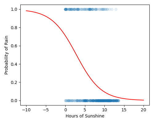
Now lets use the logistic regression model we just built on our rain data to predict whether it will rain based on the number of sunshine hours seen in the previous day. We consider the following our test data.

Sunshine	RainTomorrow
2.2	0
5.0	0
7.3	0
3.2	1
1.7	1
4.1	0
5.5	1

Instructions

1. Copy and paste in your code from Building a Logistic Regression Model

2. Create a numpy array containing the sunshine values for the days shown above

3. Use .predict to predict whether it will rain the following day (don’t forget to use .reshape(-1, 1))

4. Print the predictions

Your output should look like this:

[X X X X X X X]

By eye, verify whether your predictions are consistent with the figure shown below.

Solution

Solution is locked