4.7. KNN Regression 2D#
What we’ve looked as in KNN in 1D where there was only 1 input variable. But the same still works for if you have multiple input variables. If you have 2 input variables you can still visualise the results in 2D space.
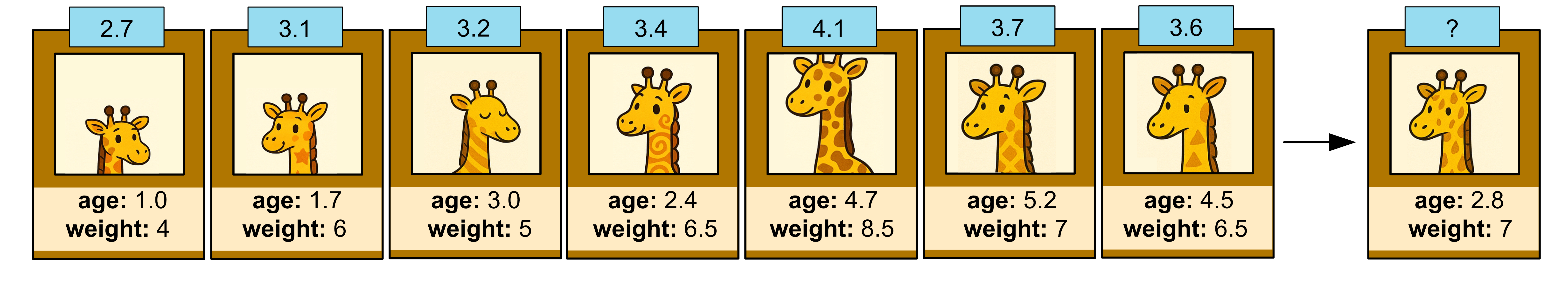
Consider the following dataset containing giraffe age, weight and heights.
Age (years) |
Height (x100kg) |
Height (cm) |
|---|---|---|
1.0 |
4 |
2.7 |
1.7 |
6 |
3.1 |
3.0 |
5 |
3.2 |
2.4 |
6.5 |
3.4 |
4.7 |
10 |
4.1 |
5.2 |
7 |
3.7 |
4.5 |
6.5 |
3.6 |
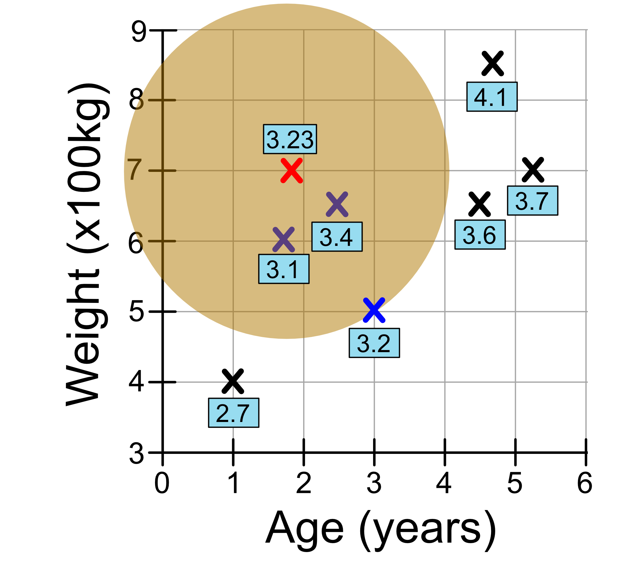
We can plot this data as shown below, including our test sample.
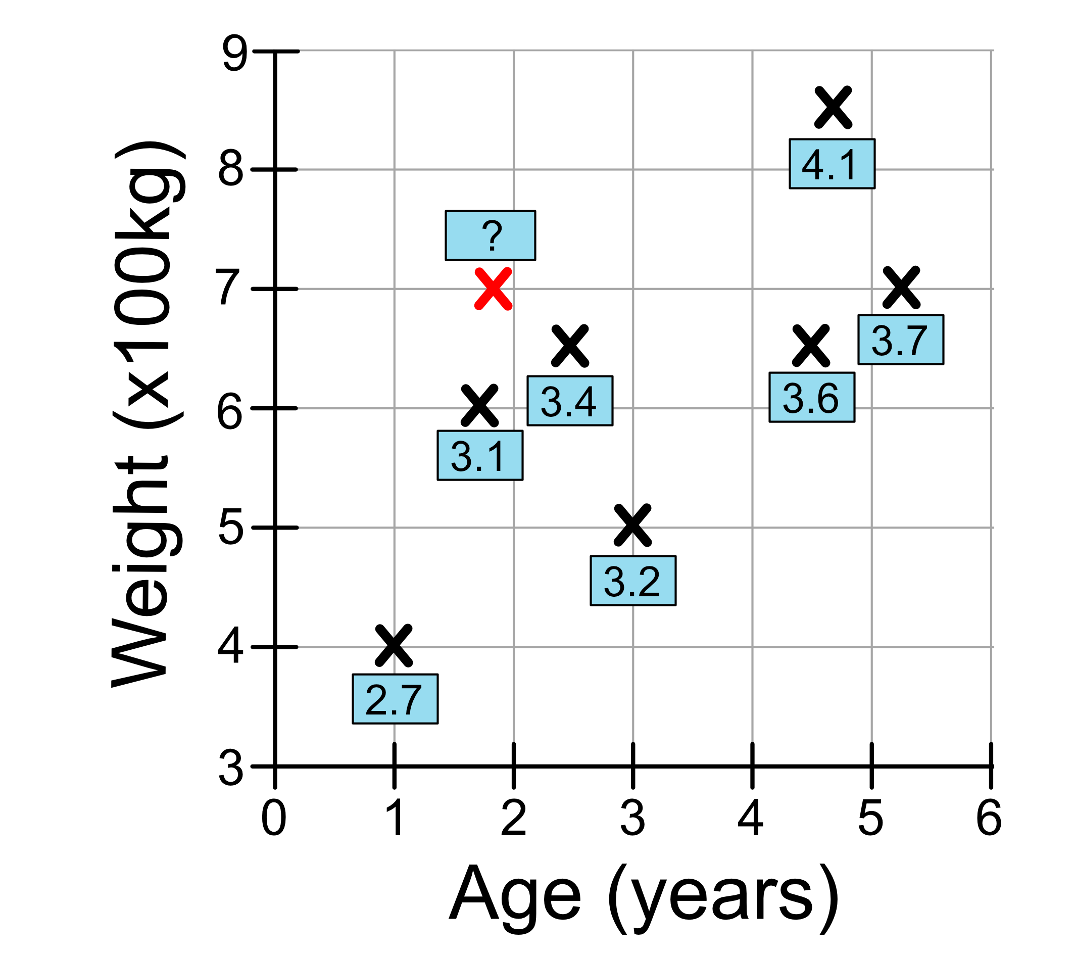
To make a prediction, we just look at the k closest neighbours. Let’s consider our test sample which is 2.8 years old and weights 7 tonnes.
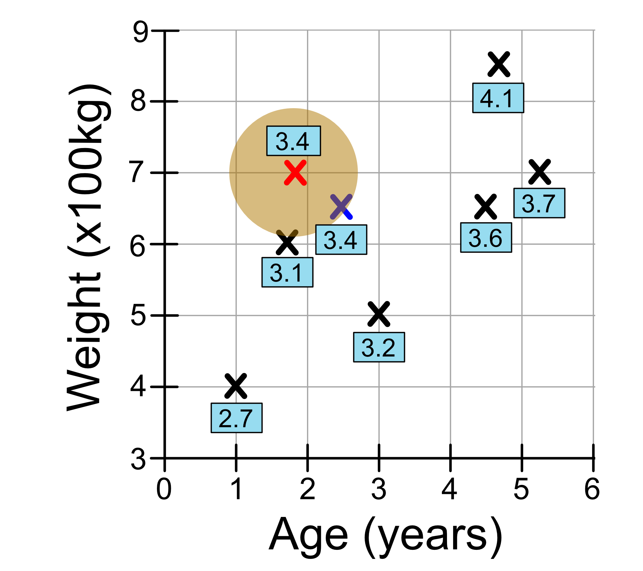
If we set k = 1, we’re just looking at our nearest neighbour. This neighbour has a height 3.4, so the prediction we make is 3.4. We’ve drawn a circle here to represent the ‘neighbourhood’. Remember that the distance from the edge of the circle to the centre is the radius. So everything inside the circle is closer than everything outside the circle.
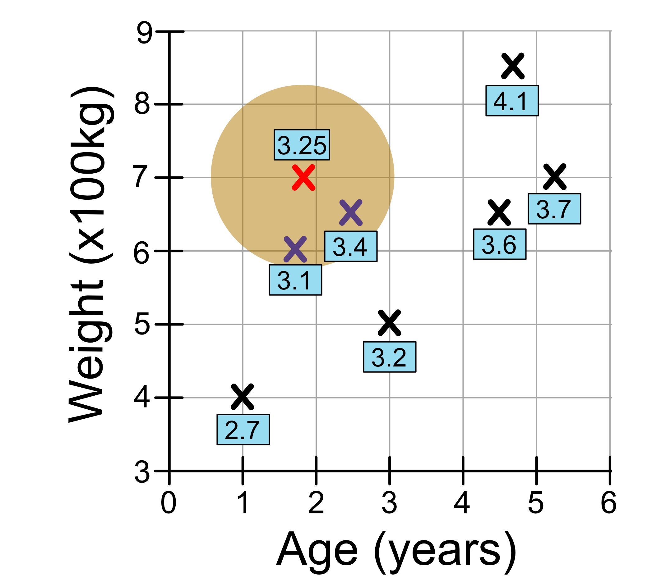
Now let’s set k = 2. We draw our circle a little bigger so we capture our two closest neighbours. This time our prediction is the average of the nearest neighbours, which is 3.25.
Now let’s set k = 3. We draw our circle a little bigger so we capture our three closest neighbours. This time our prediction is the average of the nearest neighbours, which is 3.23.
We can keep going for different values of k. And it’s up to you to decide what value of k to use.
We’ve just seen how KNN regression works for 2 input variables. It works the same for more input variables, it’s just harder to visualise. The computer is still able to calculate a distance between data points and make predictions based on the average value of the k nearest neighbours.