Making Predictions

1.11. Making Predictions#

We can make predictions using our linear regression model by estimating the $y$ value for a given $x$ value.

In our study example, we can estimate a student’s mark based on the amount of time they spent studying. For example, judging off the figure below, we would estimate that a student who has studied for 6 hours would get an exam mark of 67.

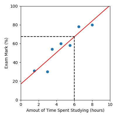
Alternatively, we can use the intercept and gradient values to calculate a prediction using the equation of the model. In this case the equation is:

\[y = 17 + 8.4x\]

Plugging in x = 6, gives us y = 17 + 8.4 \times 6 = 67.4 (Approximately, since we’re using rounded values of the intercept and gradient.)

Alternatively, our sklearn LinearRegression model comes with an in-built function that allows us to make a prediction. All we need to do is use:

linear_reg.predict(x)

Note

x must be a 2D array with n rows, one for each sample we want to predict on and 1 column. An easy way to achieve this is to use .reshape(-1, 1)

Here’s a full example:

from sklearn.linear_model import LinearRegression
import pandas as pd
import numpy as np

data = pd.read_csv("study.csv")

x = data["Time Spent Studying (hours)"].to_numpy()
y = data["Exam Mark (%)"].to_numpy()

linear_reg = LinearRegression()
linear_reg.fit(x.reshape(-1, 1), y)

x_test = np.array([6])
print(linear_reg.predict(x_test.reshape(-1, 1)))

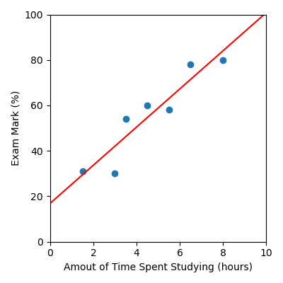
This also means that if we want to visualise our model, instead of calculating our $y$ values using the model equation $y = \beta_0 + \beta_1 x$ (as shown below):

x_model = np.linspace(0, 10, 50)
y_model = gradient * x_model + intercept

We can just use .predict(). Note that we still need to reshape the data.

x_model = np.linspace(0, 10, 50)
y_model = linear_reg.predict(x_model.reshape(-1, 1))

We have updated the code below to provide a full example. This will become more useful as we generate more complex machine learning models where the equation is not as simple as it is for our linear regression model.

from sklearn.linear_model import LinearRegression
import matplotlib.pyplot as plt
import pandas as pd
import numpy as np

# Load data
data = pd.read_csv("study.csv")
x = data["Time Spent Studying (hours)"].to_numpy()
y = data["Exam Mark (%)"].to_numpy()

# Build linear regression model
linear_reg = LinearRegression()
linear_reg.fit(x.reshape(-1, 1), y)

# Create x and y values to visualise the model function
x_model = np.linspace(0, 10, 50)
y_model = linear_reg.predict(x_model.reshape(-1, 1))

# Visualise the results
plt.figure(figsize=(4, 4))
plt.scatter(x, y)  # Data
plt.plot(x_model, y_model, color="red")  # Model
plt.xlabel("Amout of Time Spent Studying (hours)")
plt.ylabel("Exam Mark (%)")
plt.xlim([0, 10])
plt.ylim([0, 100])
plt.tight_layout()
plt.savefig("plot.png")

Code Challenge: Make A Prediction

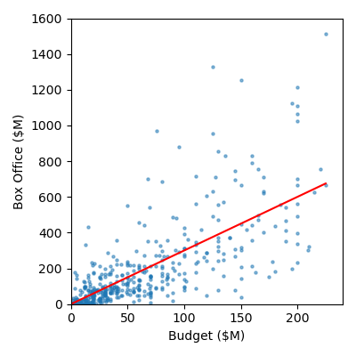
Now lets use the linear regression model we just built on our movie data movies.csv to predict the box office results for the following movies. We consider these movies our test data.

Movie	Budget ($M)
Barbie	145
Wicked	150
Everything Everywhere All At Once	25

Instructions

Copy and paste in your code from Fitting a Linear Regression Model
Create a numpy array containing the budget values for the three movies shown above
Use .predict to predict the box office results for each of these movies (don’t forget to use .reshape(-1, 1))
Print the predicted box office values

Your output should look like this:

[XXX.XXXXXXXX XXX.XXXXXXXX  XX.XXXXXXXX]

By eye, verify whether your predictions are consistent with the figure shown below.